Graphics

Plots

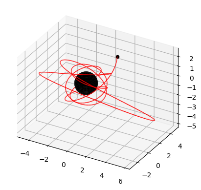
To plot an orbit, simply use the plot() method and pass in the starting and ending Mino time.

import kerrgeopy as kg
from math import pi, cos

orbit = kg.StableOrbit(0.998,3,0.6,cos(pi/4))
fig, ax = orbit.plot(0,10)

Use the initial_phases option to set the initial phases \((q_{t_0},q_{r_0},q_{\theta_0},q_{\phi_0})\) of the trajectory. For example, set \(q_{r_0} = \pi\) to start the orbit from \(r_{\text{max}}\).

fig, ax = orbit.plot(0,10, initial_phases=(0,pi,0,0))

Use the elevation and azimuth options to set the viewing angles as defined by matplotlib. To plot the orbit with a decaying tail, use the tau option to set the time constant in units of Mino time for the exponential decay in the linewidth of the tail. Use lw to adjust the initial linewidth.

orbit = kg.StableOrbit(0.999,4,0.1,cos(pi/20))
fig, ax = orbit.plot(0,10, elevation=5, lw=2, tau=5)

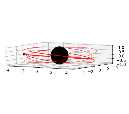
The grid and axes options can be used to turn off the visibility of the grid and axes.

orbit = kg.StableOrbit(0.999,4,0.9,cos(0))
fig, ax = orbit.plot(0,10, elevation=90, azimuth=0, grid=False, axes=False, lw=2, tau=5)

Animations

To animate an orbit, use the animate() method by passing in a filename to save the animation to, along with a starting and ending Mino time. Note that this method requires ffmpeg to be installed and may take several minutes to run depending on the length of the animation.

orbit = kg.StableOrbit(0.998,3,0.6,cos(pi/4))
orbit.animate("animation1.mp4",0,10)

All of the options available when plotting are also available within the animate() method. It is also possible to control the motion of the camera by passing in functions to set the azimuth and elevation angle in degrees as a function of Mino time.

from math import sin

orbit = kg.StableOrbit(0.998,2.1,0.8,cos(pi/20))
orbit.animate("animation2.mp4",0,20,
             elevation_pan = lambda x: 10*sin(2*pi*x/20),
             azimuthal_pan = lambda x: 360*x/20)

Use the background_color option to change the background color of the animation. If necesssary, use plt.style.use('dark_background') or with plt.style.context('dark_background'): to change the color of the grid and axes to white.

import matplotlib.pyplot as plt

orbit = kg.StableOrbit(0.999,4,0.1,cos(pi/20))
with plt.style.context('dark_background'):
    orbit.animate("animation3.mp4",0,10, background_color="black", elevation=10)

Similar to elevation_pan and azimuthal_pan, roll can be used to set the roll angle of the camera as a function of Mino time.

from math import exp

orbit = kg.StableOrbit(0.999,3,0.1,cos(pi/20))
orbit.animate("animation4.mp4", 
              elevation_pan = lambda x: 180*x/10,
              roll = lambda x: 180/(1+exp(10-2*x)),
            )

The primary black hole is always placed in the center of the plot, so the axis limits are symmetric about the origin and are the same along all three axes. To zoom in and out of the orbit, use the axis_limit option to set the axis limit as a function of Mino time. Set plot_components to True in order to plot each of the individual components of the trajectory alongside the orbit itself.

orbit = kg.StableOrbit(0.998,2.1,0.8,cos(pi/20))
t, r, theta, phi = orbit.trajectory()

with plt.style.context('dark_background'):
    orbit.animate("animation5.mp4",0,30,
                elevation = 10,
                azimuthal_pan = lambda x: 360*x/20,
                axis_limit = lambda x: r(x)+1,
                plot_components=True,
                grid=False,
                background_color="black"
                )